GOOGLE EARTH ENGINE FOR ECOLOGY AND CONSERVATION
Practical 6: Supervised learning: Landcover classification
Authored by Geethen Singh
Access the complete practical, part 1 script here
Learning Objectives
By the end of this practical you should be able to:
- Describe the workflow for a typical supervised classification workflow.
- Create reference data for classes of interest.
- Fit a random forest model on spectral variables.
- Evaluate model accuracy
The end product

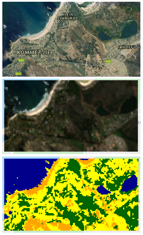
Figure 1: The distribution of water, built-up areas, tree-cover, and other (neither of the three classes) pixels at a 30 m resolution for a heterogeneous coastal area in the Western Cape, South Africa based on Landsat-8 and Sentinel-1 radar imagery.
Step 1: Import data
For this practical, you will be required to import Landsat-8 surface reflectance and Sentinel-1 Ground Range Detected imagery (GRD) data. Rename these as l8sr and s1 respectively. You have been provided with a reference points dataset (four feature collections within the imports section). However, you have the functionality to import a shapefile with reference data into GEE.
To create your own reference points
Use the following steps:
1) Click on the add Markers button.
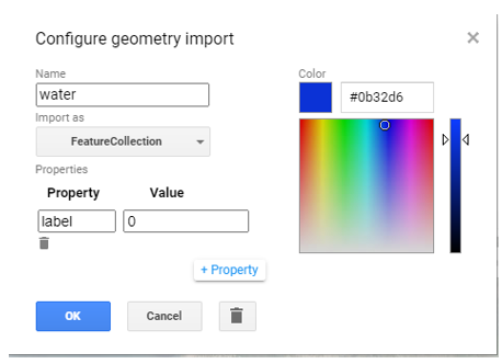
2) Hover over the geometry imports section and click on the cogwheel besides the geometry and set up the various options by
2.1) changing the ‘Name’ to the class of interest,
2.2) changing the ‘import as’ option to a feature collection,
2.3) and adding a property called label with a unique integer for each class.
3) Once set, click ok and go to the map area and add reference points for the applicable class in appropriate locations. ‘Appropriate locations’ is dependent on the spatial resolution of your imagery to be classified and the time period of interest. For instance, when working with Landsat-8, 30 m imagery, it is ideal if you add markers for areas that are dominated by the class of interest. A higher resolution base map together with an RGB or FCI can be highly useful for guiding your reference point selection. Note, use a base map that overlaps with the period of concern.

Figure 2: An example of setting up a feature collection for reference point collection of a class named water. Note, the labels for the land cover classes need to be zero-indexed (start from zero).
Step 2: Data Preparation - Filtering
Create a Landsat-8 surface reflectance composite that covers the AOI (shown by the provided geometry) for the period of 1 June 2016 to 30th September 2016, add ndvi and mndwi bands. Lastly, compute the median image, taking into consideration the GEE scaling factor and clipping to the extent of geometry.
// Scale Landsat-8 collection-2 data var scale = function(img){ var opticalBands=img.select(["SR_B.*"]).multiply(0.0000275).add(-0.2); var thermalBands=img.select("ST_B.*").multiply(0.00341802).add(149.0); return img.addBands(opticalBands,null,true) .addBands(thermalBands,null,true)}; // Create Landsat-8 composite with added spectral indices var filtered = l8sr .filterBounds(geometry) .filterDate(startDate, endDate) .map(function(image){ var ndvi = image.normalizedDifference(['B5', 'B4']).rename(['ndvi']); var mndwi = image.normalizedDifference(['B3', 'B7']).rename(['mndwi']); return image.addBands([ndvi,mndwi]); }).map(scale) .median() .clip(geometry);
Similarly, filter the Sentinel-1 data to the AOI for the period of June to September 2016 as above. In addition, filter the s1 image collection to those images that have captured in Interferometric Wide (IW) mode and contain Vertical Transmit and Vertical Receive (VV) and Vertical Transmit and Horizontal Receive polarised bands. Lastly, for each image, select all bands that start with a V and reduce the resulting images to the median image.
For more information on radar, check out:
- https://www.servirglobal.net/Global/Articles/Article/2674/sar-handbook-comprehensive-methodologies-for-forest-monitoring-and-biomass-estimation
- https://earthdata.nasa.gov/learn/backgrounders/what-is-sar
- https://developers.google.com/earth-engine/tutorials/community/sar-basics
- https://www.mdpi.com/2072-4292/13/10/1954: Create Analysis Ready Sentinel-1 data in GEE- apply terrain correction, border-noise removal and speckle filtering
var s1 = s1.filterBounds(geometry) .filterDate(startDate, endDate) .filter(ee.Filter.listContains('transmitterReceiverPolarisation', 'VV')) .filter(ee.Filter.listContains('transmitterReceiverPolarisation', 'VH')) .filter(ee.Filter.eq('instrumentMode', 'IW')) .select("V.") .median();
Create a final composite image with the bands of both the Landsat-8 composite and Sentinel-1 composite.
var composite = filtered.addBands(s1).aside(print).clip(geometry);
Step 2: Data preparation continued- preparing the train and test datasets
The next step is to split this data into a training and testing partition. The training partition is used to fit the model whilst the test data is used to evaluate the accuracy of the model. Here, we use a split of 80% train data and 20% test data. We set the seed to ensure we end up with roughly the same train and test partition when re-running the model.
//Stratified random sampling for each class var w_table = water.randomColumn({seed: 42}); var wtraining = w_table.filter(ee.Filter.lt('random', 0.80)); var wtest = w_table.filter(ee.Filter.gte('random', 0.80)); var tc_table = tree_cover.randomColumn({seed: 42}); var tctraining = tc_table.filter(ee.Filter.lt('random', 0.80)); var tctest = tc_table.filter(ee.Filter.gte('random', 0.80)); var bu_table = built_up.randomColumn({seed: 42}); var butraining = bu_table.filter(ee.Filter.lt('random', 0.80)); var butest = bu_table.filter(ee.Filter.gte('random', 0.80)); var o_table = other.randomColumn({seed: 42}); var otraining = o_table.filter(ee.Filter.lt('random', 0.80)); var otest = o_table.filter(ee.Filter.gte('random', 0.80)); //Combine land-cover reference points for training partition var training = wtraining.merge(tctraining).merge(butraining).merge(otraining).aside(print, 'training partition'); var test = wtest.merge(tctest).merge(butest).merge(otest).aside(print, 'test partition'); var points = training.merge(test).aside(print,'all points');
Depending on your goal or more specifically, the area that you intend on generalising across determines which is the most suitable way for you to do your sampling. Since we are trying to create our model for a small region, stratified random sampling will suffice. However, if you were trying to generalise across large areas then it is more suitable to use a spatially constrained cross validation technique. This will result in more reliable estimates of accuracy.
Step 2: Data preparation continued -linking the two datasets, extracting the spectral signatures
At this point, we have our response (reference points) and explanatory variables (Landsat-8 and Sentinel-1 data) prepared. We can now move on to extracting the spectral signatures at each of the points. Note, the ‘tileScale’ argument may be useful when working with large computations that fail due to computation errors.
var Features = composite.sampleRegions({ collection: training, properties: ['label'], scale: 30, tileScale:16 });
Step 3: Model fitting on training data
We fit a random forest model on the extracted spectral data for the training data partition. We choose a value of 100 for the number of trees since this is the defualt value used in pythons scikit-learn package. Choosing a larger value would increase the number of decision trees and may increase the likelihood that our model overfits to our training data. Simultaneously, selecting too few trees may result in underfitting our data and therfore less accurate land cover maps.
if you are interested in using a data-driven approach to determine the optimum number of trees - check out this hyperparameter tuning script within GEE link
var trainedClassifier = ee.Classifier.smileRandomForest(100) .train({ features: Features, classProperty: 'label', inputProperties: composite.bandNames() });
Step 4: Inference for entire AOI
var classified = composite.classify(trainedClassifier);
Step 5: Model evaluation on train and test set
The training accuracy largely overestimates model accuracy since this data has been used to train the model. We, therefore, use a test set (data unseen by the model) to get a more reliable estimate of model accuracy.
//Train accuracy var trainAccuracy = trainedClassifier.confusionMatrix().accuracy(); print('Train Accuracy', trainAccuracy); //Test accuracy var test = composite.sampleRegions({ collection: test, properties: ['label'], scale: 30, tileScale: 16 }); var Test = test.classify(trainedClassifier); print('ConfusionMatrix', Test.errorMatrix('label', 'classification')); print('TestAccuracy', Test.errorMatrix('label', 'classification').accuracy()); print('Kappa Coefficient', Test.errorMatrix('label', 'classification').kappa()); print('Producers Accuracy', Test.errorMatrix('label', 'classification').producersAccuracy()); print('Users Accuracy', Test.errorMatrix('label', 'classification').consumersAccuracy());
Visualisation
Visualising the RGB image, reference points, and classified image
Map.centerObject(points.geometry().bounds(), 13); Map.addLayer(composite,rgb_vp, 'Landsat-8 RGB');
showTrainingData(); function showTrainingData(){ var colours = ee.List(["darkblue","darkgreen","yellow", "orange"]); var lc_type = ee.List(["water", "tree cover","built-up","other"]); var lc_label = ee.List([0, 1, 2, 3]); var lc_points = ee.FeatureCollection( lc_type.map(function(lc){ var colour = colours.get(lc_type.indexOf(lc)); return points.filterMetadata("label", "equals", lc_type.indexOf(lc).add(1)) .map(function(point){ return point.set('style', {color: colour, pointShape: "diamond", pointSize: 3, width: 2, fillColor: "00000000"}); }); })).flatten(); Map.addLayer(classified, {min: 0, max: 3, palette: ["darkblue","darkgreen","yellow", "orange"]}, 'Classified image', false); Map.addLayer(lc_points.style({styleProperty: "style"}), {}, 'TrainingPoints', false); }
If you are interested in Object Based Image Analysis, check out this script. Since objects are used, some spatial context is used, performs slighly better in terms of accuracy and removes salt and pepper effect at the expense of computation.
If you are interested in Convolutional Neural Networks, check out this link
Practical 9, part 2: Supervised learning 2: Improving ypur land cover classification.
Access the complete practical, part 2 script here
Learning Objectives
By the end of this practical you should be able to:
- Understand the role and importance of high-quality training data.
- Use an objective approach (this is experimental) to improve the selection of training data.
- Determine the area of applicability for a model.
The end product

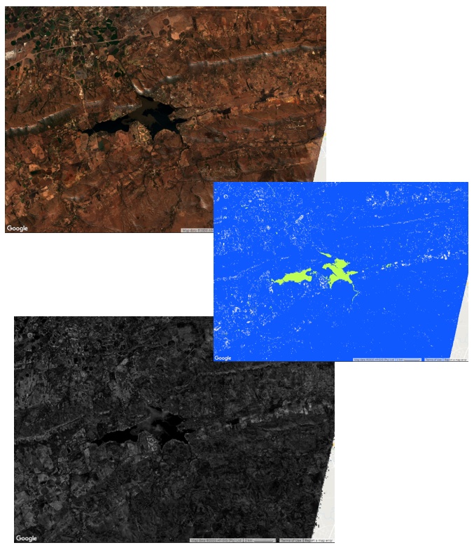
Figure 1: The area of applicability for a model that discriminated water and non-water pixels at a 10 m resolution for a heterogeneous area near Hartbeespoort Dam, South Africa based on Sentinel-2 imagery.
References
Meyer, H. and Pebesma, E., 2021. Predicting into unknown space? Estimating the area of applicability of spatial prediction models. Methods in Ecology and Evolution, 12(9), pp.1620-1633. paper here
Foody, G.M., 2020. Explaining the unsuitability of the kappa coefficient in the assessment and comparison of the accuracy of thematic maps obtained by image classification. Remote Sensing of Environment, 239, p.111630. paper here
